Description

The Laplace transform of a signal $f(t)$ is defined as $F(s)=\mathcal{L}{f(t)}=\int\_0^{\infty}f(t)e^{-st}dt$ .

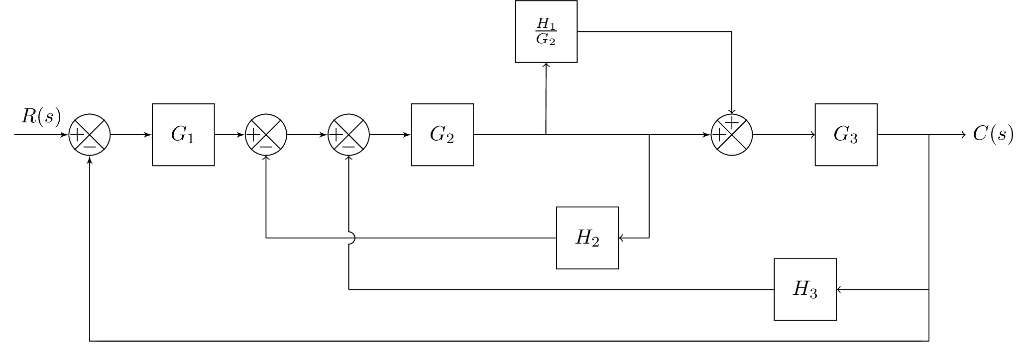
In this block diagram, $R(s)$ represents the Laplace transform of the reference input signal, $G\_1(s)$ , $G\_2(s)$ , and $G\_3(s)$ represent the transfer functions of the systems, and $H\_1(s)$ , $H\_2(s)$ , and $H\_3(s)$ represent the transfer functions of the feedback paths.

The block diagram can be represented mathematically as: $C(s)=G\_3(s)(R(s)-G\_2(s)H\_1(s)C(s))-G\_1(s)H\_2(s)C(s)$

The signal flow through the diagram is as follows: The reference input $R(s)$ is fed to the summing junction where it is added to the feedback signal $-G\_2(s)H\_1(s)C(s)$ to produce the error signal. The error signal is then fed through the transfer function $G\_3(s)$ to produce the output signal $C(s)$ .

The feedback signal is also fed through the transfer function $H\_2(s)$ and then added to the output of $G\_1(s)$ . The resulting signal is then fed through the transfer function $H\_3(s)$ and subtracted from the error signal at the summing junction.

Keywords

tikz, nodes, arrows, styles, positioning, shapes.

Source Code

ControlSystems/CSI

% standalone diagram for block diagrams
\documentclass{standalone}
 
\usepackage{blox}
\usepackage{tikz}
\usetikzlibrary{positioning}
\newcommand{\equal}{=}
\usepackage{tikz}
\usetikzlibrary{intersections}
\usepackage{tkz-euclide}
% Radius for arc over intersection
\def\radius{1.mm} 
 
\tikzset{
	connect/.style args={(#1) to (#2) over (#3) by #4}{
		insert path={
			let \p1=($(#1)-(#3)$), \n1={veclen(\x1,\y1)}, 
			\n2={atan2(\y1,\x1)}, \n3={abs(#4)}, \n4={#4>0 ?180:-180}  in 
			(#1) -- ($(#1)!\n1-\n3!(#3)$) 
			arc (\n2:\n2+\n4:\n3) -- (#2)
		}
	},
}
 
\begin{document}
\begin{tikzpicture}
\bXInput{A}				% Input
\bXComp{B}{A}			% First adder
\bXLink[$R(s)$]{A}{B}	% Input Label
\bXBloc[2]{C}{$G_1$}{B}	% Block G1
\bXLink{B}{C}			% First added -- G1
\bXComp{D}{C}			% Second adder
\bXComp{E}{D}			% Third adder
\bXBloc[2]{G2}{$G_2$}{E}	% Block G2
\bXBranchx[5]{G2}{G2Right}	% Branch for H1, G2
\bXBranchy[-5]{G2Right}{invG2H1Left}	% node before 1 /G2
\bXBloc[-1.5]{invG2H1}{$\frac{H_1}{G_2}$}{invG2H1Left}	% Block 1/G2
\bXBranchx[-3.5]{invG2H1}{invG2H1left}	% Branch for H1, G2
 
\bXBranchx[10]{G2}{Bran2}		% Branch after G2 and for H2
\bXBranchy[5]{Bran2}{Bran2Down}	% beneath branch 2
\bXBloc[-4.5]{H2Block}{$H_2$}{Bran2Down}
\bXSuma{adder4}{Bran2}
\bXLink{C}{D}
\bXLink{D}{E}
\bXLink{E}{G2}
\bXLink{G2}{adder4}		% G2 to adder
 
\bXBloc[3]{G3Block}{$G_3$}{adder4} % G3
\bXBranchx[4]{G3Block}{BranEnd} % branch before output
\bXBranchy[7.5]{BranEnd}{H3BlockRight} % Right H3 Block
\bXBranchy[2.5]{H3BlockRight}{BranEndReturn} % Right H3 Block
\bXBranchy[7.5]{E}{adder3down} % Below adder3
\bXBloc[-7.5]{H3Block}{$H_3$}{H3BlockRight}	% H3 Block
\draw[-] (BranEnd.center) -- (H3BlockRight.center);
\draw[->] (H3BlockRight.center) -- (H3Block);
\draw[-] (H3BlockRight.center) -- (BranEndReturn.center);
\bXBranchy[10]{B}{adder1Down}
\draw[-] (BranEndReturn.center) -- (adder1Down);
 
\bXBranchy[5]{D}{adder2down}	% beneath adder2
\bXBranchy[-5]{adder4}{adder4up}		% beneath adder4
%\bXLinkyx{EH1.center}{H2} % -- Connection for branch 1 and H1
\draw[->]  (G2Right.center) -- (invG2H1);
%\draw[->] (invG2) -- (H1);
\draw[->] (Bran2Down.center) -- (H2Block);
\draw[-] (Bran2Down.center) -- (Bran2.center);
\draw[-,name path=H2 to adder2down] (H2Block) -- (adder2down.center); % used in intersection
\draw[->] (adder2down.center) -- (D);
\draw[-]  (invG2H1) -- (adder4up.center);
\draw[->]  (adder4up.center)   -- (adder4);
\draw[->] (adder4) -- (G3Block);
 
\node[right = 0.5cm of BranEnd] (end) {$C(s)$};
\draw[->] (G3Block) -- (end);
 
\draw[-] (H3Block) -- (adder3down.center);
\path[name path=line] (adder3down.center) -- (E);
\path[name intersections={of=H2 to adder2down and line,by=inter}];
\draw[->,connect=(adder3down.center) to (E) over (inter) by 3pt ];
 
\bXLinkxy{BranEndReturn}{B}
 
\end{tikzpicture}
\end{document}

Deploy to Overleaf

Q5blockdiagram2 Q5blockdiagram3