Description
This is a LaTeX document that uses the standalone class and loads several packages including tikz, pgfplots, filecontents, and amsmath. The data for the plot is contained in an external file named data.dat, which is defined using the filecontents package.
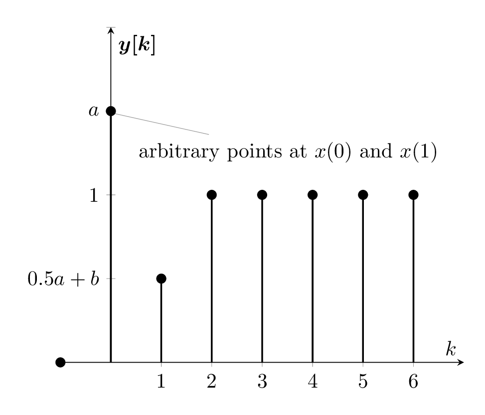
The main part of the code is a tikzpicture environment with an axis environment inside it. The axis environment is configured to have a middle x and y axis, x and y labels, and specific x and y tick labels. The ycomb plot style is used to draw a thick black line connecting the data points from the data.dat file. An additional plot is added with a single point at the coordinate (0,5.825) with a text label below it reading "arbitrary points at and ".
Overall, this code generates a plot of discrete data points with tick labels and an additional point with a label.
Keywords
tikzpicture, axis, axis x line, axis y line, every axis x label, every axis plot post, xlabel, ylabel, xtick, xmax, ymin, ymax, yticklabels, addplot, ycomb, table, coordinates, node, pin.
Source Code
\documentclass[border={10pt}]{standalone}
\usepackage{tikz,pgfplots,filecontents,amsmath}
\pgfplotsset{compat=1.5}

\begin{filecontents}{data.dat}
 n   yn
-1   0
0    6
1    2
2    4
3    4
4    4
5    4
6    4
\end{filecontents}


\begin{document}
\begin{tikzpicture}
\begin{axis}
[%%%%%%%%%%%%%%%%%%%%%%%%%%%%%%%%%%%
    axis x line=middle,
    axis y line=middle,
    every axis x label={at={(current axis.right of origin)},anchor=north west},
    %every axis y label={at={(current axis.above origin)},anchor= north west},
    every axis plot post/.style={mark options={fill=black}},
    xlabel={$k$},
    ylabel={$\boldsymbol{y[k]}$},
    xtick={0,1, ..., 6},
    xmax=7,
    ymin=0,
    ymax=8,
    yticklabels={
    	$0$,
    	$0$,
    	$0.5a+b$,
    	$1$,
    	$a$
    },
]%%%%%%%%%%%%%%%%%%%%%%%%%%%%%%%%%%%
\addplot+[ycomb,black,thick] table [x={n}, y={yn}] {data.dat};
%\addplot[mark=*] coordinates {(1,2)} node[pin=45:{}]{} ;
\addplot[] coordinates {(0,5.825)} node[pin=320:{arbitrary points at $x(0)$ and $x(1)$}]{} ;
\end{axis}
\end{tikzpicture}

\end{document}