Description
The code is a LaTeX document that uses the standalone document class to create a standalone image of an electrical circuit diagram. The document loads several packages, including circuitikz for drawing circuit diagrams, graphicx for including graphics, mathrsfs for special math symbols, and amssymb, amsmath, and latexsym for mathematical typesetting.
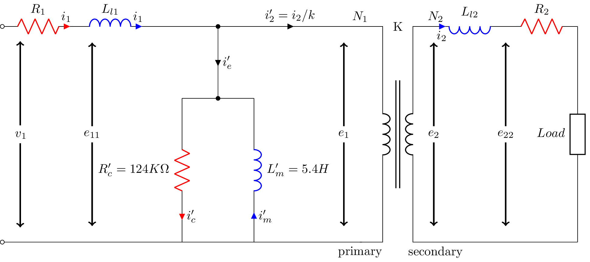
The circuit diagram is defined within a circuitikz environment, and consists of several components including resistors, inductors, transformers, and a load. The diagram includes labels for the various components and arrows indicating the direction of current flow.
The code also defines several coordinate points and nodes, which are used to place labels on the diagram and draw arrows to indicate voltage drops.
Overall, the code generates a detailed and labeled electrical circuit diagram that can be used in various documents, presentations, or reports.
Keywords
tikzpicture, node, draw, circle, right, below, edge, label, style
Source Code
\documentclass{standalone}
\usepackage[american]{circuitikz}
\usetikzlibrary{calc,arrows}
\usepackage{graphicx}
\usepackage{mathrsfs}
\usepackage{latexsym,amssymb,amsmath}
\newcommand{\equal}{=}
\begin{document}
	\begin{circuitikz}
		\draw (0,6) to [open,l=$v_1$,o-o] (0,0)
		(0,6) to  [R,i>=$i_1$, l^= $R_{1}$, color=red] (2,6)
		(2,6) to  [L,i>=$i_1$,l^= $L_{l1}$, color=blue] (4,6)
		(4,6) -- (6,6)
		(6,6) to [short,i=$i^\prime_e$,*-*] (6,4)
		(6,4) -- (5,4)
		(6,4) -- (7,4)
		(5,4) to [R,i^>=$i^\prime_c$, l_= $R^{\prime}_c\equal 124K \Omega$, color=red] (5,0)
		(7,4) to [L,i^<=$i^\prime_m$, l^= $L^{\prime}_m \equal 5.4 H$, color=blue] (7,0)
		(6,6) to [short,i=$i^\prime_2 \equal i_2 / k$] (10,6)
		(0,0) -- (10,0)
		(11,6) node [yscale =2.857,transformer core](T){}  % reminded by @PaulGessler, thanks.
		(T.A1) node[above] {$N_1$}
		(T.A2) node[below] {primary}
		(T.B1) node[above] {$N_2$}
		(T.B2) node[below] {secondary}
		(T.base) node{K}

		(T.B1) -- (12,6)
		(14,6) to [L,i^<=$i_2$, l_= $L_{l2}$, color=blue] (12,6)
		(14,6) to [R, l^= $R_{2}$, color=red] (16,6)
		(16,6) to [generic, l_=${Load}$](16,0)
		(T.B2) -- (16,0)
%	    (4,0) -- (0,0)
%	     (4,4) to [R,i^>=$\phi_2$, l^= $\mathscr{R}_{2}$,v_>=$\mathscr{F}_2$, color=blue] (4,0)
%		(4,4) to [R,l^= $\mathscr{R}_{3}$,v_>=$\mathscr{F}_3$, color=red] (8,4)
%		(8,4) to [R,i^>=$\phi_3$, l^= $\mathscr{R}_{g}$,v_>=$\mathscr{F}_g$, color=cyan] (8,0)
%		(8,0) to [R, l^= $\mathscr{R}_{4}$,v_>=$\mathscr{F}_4$, color=green] (4,0);
%		\draw[thin, <-, >=triangle 45] (6,2) node{$\phi_3$}   ++(-90:1) arc (-90:100:1);
%		\draw[thin, <-, >=triangle 45] (2,2) node{$\phi_2$}   ++(-90:1) arc (-90:100:1);
%		\node (phi) at (4.25,0.5) {$\phi_2$};
%		\draw[-stealth]  (4.25,2.5) to [bend left=90] (phi);
;
\coordinate (V1up) at (0.5,6);
\coordinate (V1mid1) at (0.5,3.25);
\coordinate (V1mid2) at (0.5,2.75);
\coordinate (V1down) at (0.5,0);
\node (e) at (2.5,3) {$e_{11}$};
\node (eend) at (9.5,3) {$e_{1}$};
\node (e2) at (12,3) {$e_{2}$};
\node (e3) at (14,3) {$e_{22}$};
\draw[->,black,very thick] (e) -- ($(e)!.85!(2.5,6)$); % 1 cm before end terminal
\draw[->,black,very thick] (e) -- ($(e)!.85!(2.5,0)$); % 1 cm before start terminal
\draw[->,black,very thick] (eend) -- ($(eend)!.85!(9.5,6)$); % 1 cm before end terminal
\draw[->,black,very thick] (eend) -- ($(eend)!.85!(9.5,0)$); % 1 cm before start terminal
\draw[->,black,very thick] (e2) -- ($(e2)!.85!(12,6)$); % 1 cm before end terminal
\draw[->,black,very thick] (e2) -- ($(e2)!.85!(12,0)$); % 1 cm before start terminal
\draw[->,black,very thick] (e3) -- ($(e3)!.85!(14,6)$); % 1 cm before end terminal
\draw[->,black,very thick] (e3) -- ($(e3)!.85!(14,0)$); % 1 cm before start terminal
\draw[->,black,very thick] (V1mid2) -- ($(V1mid2)!.85!(V1down)$); % 1 cm before end terminal
\draw[->,black,very thick] (V1mid1) -- ($(V1mid1)!.85!(V1up)$); % 1 cm before start terminal
	\end{circuitikz}
	\label{fig:q1fig}
\end{document}