Description
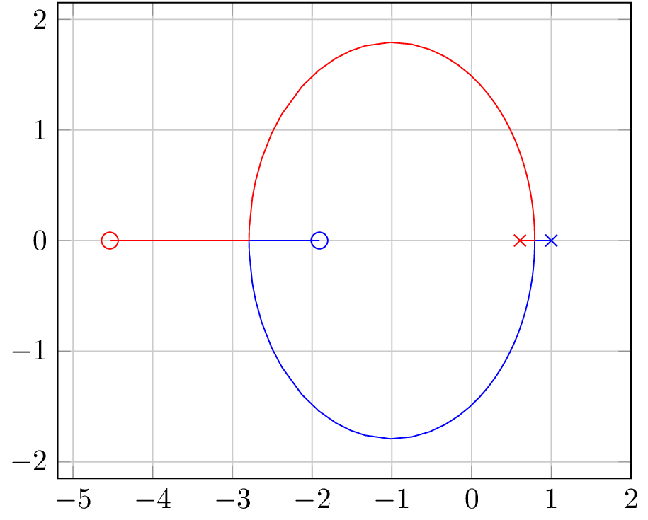
The code appears to be generating a plot of root loci for a digital control system as the gain is varied from to . The plot shows how the poles and zeros of the system change as the gain is increased. The root locus plot is a useful tool for analyzing and designing feedback control systems.
The plot seems to be generated using the Matlab software and exported in the TikZ format, which is used for creating high-quality graphics in LaTeX documents. The plot shows the imaginary and real parts of the poles and zeros of the system as they move along the root locus. The root locus indicates the range of gain values for which the system is stable, and also provides information about the transient and steady-state responses of the system.
Overall, the plot provides a useful visual representation of the behavior of the control system, and can be used to analyze the stability and performance of the system.
Keywords
tikz, pgf, nodes, shapes, arrows, positioning, styles
Source Code
   % Plot generated in matlab for the following question
   % question: Consider the digital control system Plot the root loci as the gain K is varied from $0$ to $\infty$.

   \documentclass{standalone}
   \usepackage{pgfplots}
   % Manually removed entries to plot a "better" root locus in latex, of course using matlab 2 tikz is much better.
   \pgfplotsset{compat=1.11}
   \pgfplotstableread{
   	pr1 		 pi1 	  pr2 		pi2 		k
    1.0000         0    0.6065         0         0
    0.9272         0    0.6672         0    0.0121
    0.9109         0    0.6814         0    0.0142
    0.8887         0    0.7011         0    0.0166
    0.8541         0    0.7329         0    0.0195
    0.7987         0    0.7863         0    0.0215
    0.7925   -0.0000    0.7925    0.0000    0.0215
    0.7925   -0.0062    0.7925    0.0062    0.0216
    0.7918   -0.0482    0.7918    0.0482    0.0228
    0.7899   -0.0967    0.7899    0.0967    0.0268
    0.7876   -0.1326    0.7876    0.1326    0.0313
    0.7849   -0.1649    0.7849    0.1649    0.0367
    0.7817   -0.1961    0.7817    0.1961    0.0430
    0.7780   -0.2272    0.7780    0.2272    0.0504
    0.7737   -0.2588    0.7737    0.2588    0.0591
    0.7686   -0.2915    0.7686    0.2915    0.0693
    0.7627   -0.3255    0.7627    0.3255    0.0812
    0.7557   -0.3613    0.7557    0.3613    0.0951
    0.7475   -0.3989    0.7475    0.3989    0.1114
    0.7380   -0.4387    0.7380    0.4387    0.1306
    0.7267   -0.4810    0.7267    0.4810    0.1530
    0.7136   -0.5259    0.7136    0.5259    0.1793
    0.6982   -0.5737    0.6982    0.5737    0.2101
    0.6802   -0.6245    0.6802    0.6245    0.2462
    0.6590   -0.6787    0.6590    0.6787    0.2885
    0.6342   -0.7364    0.6342    0.7364    0.3380
    0.6052   -0.7977    0.6052    0.7977    0.3961
    0.5712   -0.8628    0.5712    0.8628    0.4641
    0.5313   -0.9317    0.5313    0.9317    0.5439
    0.4846   -1.0045    0.4846    1.0045    0.6373
    0.4299   -1.0810    0.4299    1.0810    0.7468
    0.3657   -1.1610    0.3657    1.1610    0.8751
    0.2906   -1.2440    0.2906    1.2440    1.0254
    0.2025   -1.3293    0.2025    1.3293    1.2015
    0.0993   -1.4158    0.0993    1.4158    1.4079
    -0.0217   -1.5019   -0.0217    1.5019    1.6498
    -0.1634   -1.5853   -0.1634    1.5853    1.9332
    -0.3294   -1.6623   -0.3294    1.6623    2.2653
    -0.5240   -1.7281   -0.5240    1.7281    2.6545
    -0.7520   -1.7752   -0.7520    1.7752    3.1105
    -1.0192   -1.7924   -1.0192    1.7924    3.6449
    -1.3323   -1.7614   -1.3323    1.7614    4.2710
    -1.5157   -1.7167   -1.5157    1.7167    4.6379
    -1.6991   -1.6505   -1.6991    1.6505    5.0047
    -1.9140   -1.5419   -1.9140    1.5419    5.4346
    -2.1290   -1.3923   -2.1290    1.3923    5.8645
    -2.3809   -1.1429   -2.3809    1.1429    6.3682
    -2.5068   -0.9709   -2.5068    0.9709    6.6201
    -2.6327   -0.7398   -2.6327    0.7398    6.8719
    -2.7108   -0.5349   -2.7108    0.5349    7.0281
    -2.7498   -0.3886   -2.7498    0.3886    7.1062
    -2.7889   -0.1135   -2.7889    0.1135    7.1843
    -2.7925   -0.0000   -2.7925    0.0000    7.1915
    -2.6825         0   -2.9097         0    7.1987
    -1.9082         0   -4.5377         0    8.0524
}\mytable

\begin{document}

\begin{tikzpicture}[
%This is to provide the start  point cross marker
start marker/.pic={\draw (-#1,-#1) -- (#1,#1) (#1,-#1)--(-#1,#1);}
]
\begin{axis}[no marks,xmax=2,grid=both]% Don't put any markers, limit the visible area from one side ,draw grid
\foreach\x in{1,...,2}{% Iterate over the columns of the table
	\addplot+[] table[x=pr\x,y=pi\x] {\mytable} % Draw the curves
	node[draw,circle,inner sep=2pt] at (current plot end) {}%Put the ending marker with size adjusted to 2pt
	pic at (current plot begin) {start marker=2pt};%Put the starting marker
}
\end{axis}
\end{tikzpicture}
\end{document}