Description
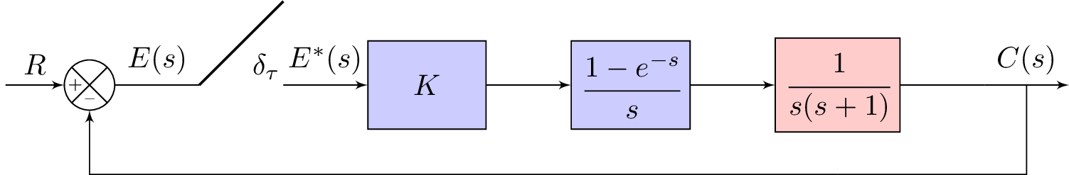
This is a LaTeX code for drawing a block diagram using TikZ package. The diagram represents a control system with a feedback loop. The system consists of several blocks, including a summing point, a gain block, a zero-order hold block, and a controller block. The input signal is represented by the symbol "R", while the output signal is represented by the symbol "C(s)". The feedback loop is closed by connecting the output of the controller block to the summing point.
The code defines various styles for the blocks, including the input and output nodes, the summing point, the gain block, the zero-order hold block, and the controller block. The TikZ library "positioning" is used to position the blocks relative to each other. The "add" style is defined to create a customized circle node with four small nodes representing plus and minus signs.
The diagram is drawn using the TikZ environment "tikzpicture". The various blocks are drawn as nodes and connected using arrows. The "draw" and "fill" commands are used to define the appearance of the blocks. The "node" command is used to label the input and output signals, as well as to add text to the various blocks. The "draw" and "fill" styles are used to define the appearance of the connecting arrows.
Overall, this code creates a visual representation of a control system that can be used in academic and engineering contexts.
Keywords
documentclass, standalone, usepackage, tikz, amsmath, usetikzlibrary, positioning, shapes, arrows, calc, decorations.text, tikzset.
Source Code
\documentclass[%
% border=1pt
border={-25pt 0pt 0pt 0pt} % left bottom right top
]{standalone}
\usepackage{tikz}
\usepackage{amsmath}
\usetikzlibrary{positioning}
\usetikzlibrary{shapes,arrows,calc}
\usetikzlibrary{decorations.text}
\tikzset{add/.style n args={4}{
		minimum width=6mm,
		path picture={
			\draw[black]
			(path picture bounding box.south east) -- (path picture bounding box.north west)
			(path picture bounding box.south west) -- (path picture bounding box.north east);
			\node at ($(path picture bounding box.south)+(0,0.13)$)     {\tiny #1};
			\node at ($(path picture bounding box.west)+(0.13,0)$)      {\tiny #2};
			\node at ($(path picture bounding box.north)+(0,-0.13)$)        {\tiny #3};
			\node at ($(path picture bounding box.east)+(-0.13,0)$)     {\tiny #4};
		}
	}
}
\begin{document}

%\begin{figure}
%\centering
	\tikzstyle{block} = [draw, fill=blue!20, rectangle, minimum height=3em, minimum width=4em]
	\tikzstyle{controller} = [draw, fill=red!20, rectangle, minimum height=3em, minimum width=4em]
	\tikzstyle{sum} = [draw, fill=blue!20, circle, node distance=1cm]
	\tikzstyle{input} = [coordinate]
	\tikzstyle{output} = [coordinate]
	\tikzstyle{sampleSP} = [coordinate]
	\tikzstyle{sampleEP} = [coordinate]
	\tikzstyle{otherPoint} = [coordinate]
	\begin{tikzpicture}[auto, >=latex']
	% Nodes
	\node [input] (input) {};
	%\node [sum, right = 1cm of input] (sum) {};
	\node[draw,circle,add={--}{+}{}{},right of= input](sum){};
	\node [sampleSP, right = 1cm of sum] (sumSP) {};
	\node [sampleEP, right = 1cm of sumSP] (sumEP) {};
	\node [sampleEP, above = 1cm of sumEP] (sumEPTOP) {};
	\node [block, right = 1cm of sumEP] (systemK) {$K$};
	\node [block, right = 1cm of systemK] (systemZOH) {$\cfrac{1-e^{-s}}{s}$};
	\node [controller, right = 1cm of systemZOH] (system) {$\cfrac{1}{s(s+1)}$};
	\node [otherPoint,right = 1cm of system] (branchPoint) {};
	\node [otherPoint,below = 1 cm of system] (belowsystem) {}; %{$\frac{1}{Ts+1}$};
	%\node [block, right = 1cm of system] (system2) {$\frac{1}{Ts+1}$};
	\node [output, right = 1cm of branchPoint] (output) {};
	\node [input, below = 0.5cm of system] (m) {};

	% Arrows
	\draw [draw,->] (input) -- node {$R$} (sum);
	% Arrows for first sampler
	\draw [-] (sum) -- node {$E(s)$} (sumSP);
	\draw [-,thick] (sumEPTOP) -- node {$\delta_\tau$} (sumSP);
	\draw [->] (sumEP) -- node {$E^\ast(s)$} (systemK);
	\draw [->] (systemK) -- node {} (systemZOH);
	\draw [->] (systemZOH) -- node {} (system);
	%\draw [->] (sumEP) -- node {$M^\ast(s)$} (systemH);
	% \draw [->] (system) --  (system2);
	\draw [-] (system) --  (branchPoint);
	\draw [->] (branchPoint) -- node (y) {$C(s)$}(output);

	\draw [-] (y) |- (m) {} ;
	\draw [->] (m) -| (sum); %{$-$}  node [near end] {} (sum);
	\end{tikzpicture}
%\end{figure}
\end{document}