Description
This is a LaTeX code for a diagram using the TikZ package. The document class is set to article and the geometry package is used to set the paper size and margins. The bm and eucal packages are also used for mathematical symbols and fonts.
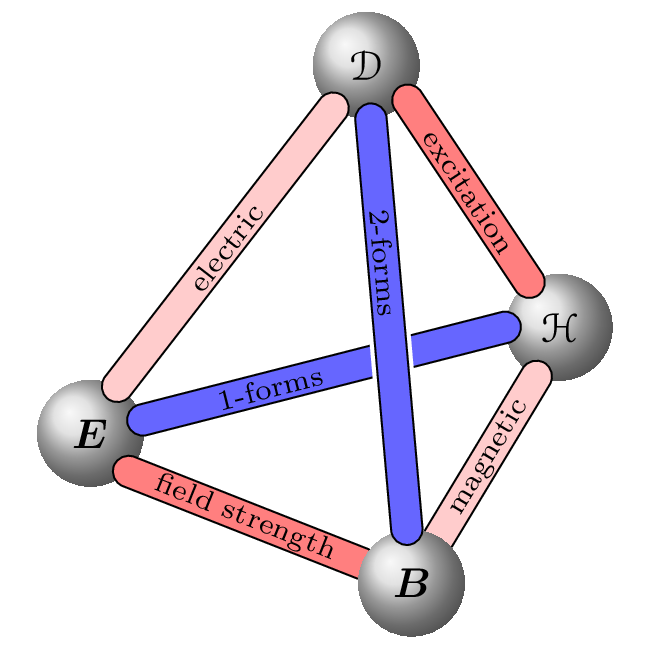
The diagram shows four balls labeled B, D, E, and H which represent physical concepts in electromagnetism. Each ball is defined as a circle with shading and a minimum size. The TikZ library decorations.markings is used to add labels to the connections between the balls.
There are several custom macros defined in the code, such as \conline and \connectpos, which are used to draw connections between the balls with specific styles and labels. The code also uses the TikZ library calc to calculate the positions of some of the balls.
Overall, the code is defining a diagram that visually represents the relationships between different concepts in electromagnetism.
Keywords
Keywords: TikZ, geometry, bm, eucal, ball, circle, shading, minimum size, decorations.markings, label, blue, red, postaction, transform shape, decoration, markings, mark, color, line width, line cap, round, node, execute, begin scope, end scope, layer, zlevel, main, conline, connectpos, connection, calc, centering, scope.
Source Code
\documentclass{article}
\usepackage[paperwidth=55mm,paperheight=55mm,margin=1mm]{geometry}
\usepackage{bm}
\usepackage{eucal}
\usepackage{tikz}
\usetikzlibrary{calc}
\usetikzlibrary{decorations.markings}
\pagestyle{empty}
\parindent=0pt
\begin{document}
\pgfdeclarelayer{-1}
\pgfsetlayers{-1,main}
\tikzset{
    zlevel/.style={%
        execute at begin scope={\pgfonlayer{#1}},
        execute at end scope={\endpgfonlayer}
    },
}
\centering
\begin{tikzpicture}[
        ball/.style={circle, shading=ball, ball color=black!15, minimum size=9mm},
        conline/.style={line width=#1, line cap=round},
        label/.style 2 args={
            postaction={decorate,transform shape,decoration={
                markings, mark=at position #1 with \node {\scriptsize\color{black}#2};
            }}
        },
        blue/.style={color=blue!60},
        red/.style={color=red!50},
        redl/.style={color=red!20},
    ]
    \def\conline<#1>[#2] (#3) (#4);{%
        \draw[conline=#1, #2] (#3) -- (#4);
    }
    \def\conwhiline (#1) (#2);{%
        \conline<10pt>[color=white] (#1) (#2);
    }
    \def\connectpos[#1] (#2) (#3) #4 #5;{%
        \conline<8pt>[color=black] (#2) (#3);
        \conline<7pt>[#1, label={#4}{#5}] (#2) (#3);
    }
    \def\connection[#1] (#2) (#3) #4;{%
        \connectpos[#1] (#2) (#3) 0.5 {#4};
    }
    \node (B) [ball]                     {$\bm{B}$};
    \node (D) [ball] at ($(B)+(95:4.4)$) {$\mathcal{D}$};

    \begin{scope}[zlevel=-1]
    \node (H) [ball] at ($(B)+(60:2.5)$) {$\mathcal{H}$};
    \node (E) [ball] at ($(B)+(155:3)$)  {$\bm{E}$};
    \connectpos[blue] (E)     (H.180) 0.35 {1-forms};
    \conwhiline       (B)     (D);
    \connection[red]  (E.-45) (B)          {field strength};
    \connection[redl] (B)     (H.-115)     {magnetic};
    \end{scope}

    \connection[red]  (D.-40) (H)          {excitation};
    \connectpos[blue] (D)     (B)     0.35 {2-forms};
    \connection[redl] (E.60)  (D)          {electric};
\end{tikzpicture}
\end{document}