Description
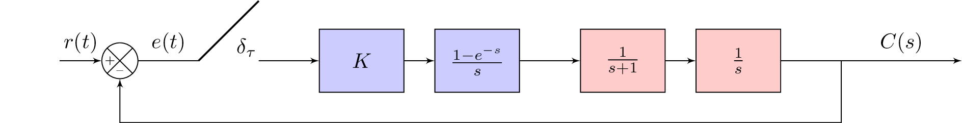
The code is a LaTeX document that creates a block diagram using TikZ library. The block diagram represents a control system with various blocks, each block represented as a rectangle with text inside it. The lines connecting the blocks represent signals flowing from one block to another. The lines can be solid, dashed, or dotted, and they have arrows indicating the direction of the signal flow. The code also uses the "add" style to add a crosshair to a circle node. The code defines several TikZ styles for nodes with different shapes and colors, including "block", "controller", "sum", "input", "output", "sampleSP", "sampleEP", and "otherPoint". The code places the nodes in the block diagram using the "positioning" library, which allows the nodes to be positioned relative to each other. The nodes are connected using the "auto" option to automatically position the arrows without overlapping. The code also includes comments to describe what each line of code does.
Keywords
tikzpicture, node, rectangle, draw, fill, below, right, of.
Source Code
\documentclass{standalone}
\usepackage{tikz}
\usetikzlibrary{positioning}
\usetikzlibrary{shapes,arrows,calc}
\usetikzlibrary{decorations.text}
\tikzset{add/.style n args={4}{
		minimum width=6mm,
		path picture={
			\draw[black]
			(path picture bounding box.south east) -- (path picture bounding box.north west)
			(path picture bounding box.south west) -- (path picture bounding box.north east);
			\node at ($(path picture bounding box.south)+(0,0.13)$)     {\tiny #1};
			\node at ($(path picture bounding box.west)+(0.13,0)$)      {\tiny #2};
			\node at ($(path picture bounding box.north)+(0,-0.13)$)        {\tiny #3};
			\node at ($(path picture bounding box.east)+(-0.13,0)$)     {\tiny #4};
		}
	}
}
\begin{document}

%\begin{figure}
%\centering
	\tikzstyle{block} = [draw, fill=blue!20, rectangle, minimum height=3em, minimum width=4em]
	\tikzstyle{controller} = [draw, fill=red!20, rectangle, minimum height=3em, minimum width=4em]
	\tikzstyle{sum} = [draw, fill=blue!20, circle, node distance=1cm]
	\tikzstyle{input} = [coordinate]
	\tikzstyle{output} = [coordinate]
	\tikzstyle{sampleSP} = [coordinate]
	\tikzstyle{sampleEP} = [coordinate]
	\tikzstyle{otherPoint} = [coordinate]
	\begin{tikzpicture}[auto, >=latex']
	% Nodes
	\node [input] (input) {};
	%\node [sum, right = 1cm of input] (sum) {};
	\node[draw,circle,add={--}{+}{}{},right of= input](sum){};
	\node [sampleSP, right = 1cm of sum] (sumSP) {};
	\node [sampleEP, right = 1cm of sumSP] (sumEP) {};
	\node [sampleEP, above = 1cm of sumEP] (sumEPTOP) {};
	\node [block, right = 1 cm of sumEP] (systemK) {$K$};
	\node [block, right = 0.5 cm of systemK] (system2) {$\frac{1-e^{-s}}{s}$};
	\node [controller, right = 1 cm of system2] (system3) {$\frac{1}{s+1}$};
	\node [controller, right = 0.5 cm of system3] (systemEND) {$\frac{1}{s}$};
	\node [otherPoint,right = 1 cm of systemEND] (branchPoint) {};
	\node [otherPoint,below = 1 cm of systemEND] (belowsystem) {}; %{$\frac{1}{Ts+1}$};
	%\node [block, right = 1cm of system] (system2) {$\frac{1}{Ts+1}$};
	\node [output, right = 2cm of branchPoint] (outputY) {};
	\node [input, below = 0.5cm of systemEND] (m) {};
%	\node [block, right = 0.75 of belowsystem] (systemH) {$H_1(s)$};

	% Second Sampler Point
%	\node [sampleSP, left = 1cm of systemH] (sysHSP2) {};
%	\node [sampleEP, left = 1cm of sysHSP2] (sysHEP2) {};
%	\node [sampleEP, above = 1cm of sysHEP2] (sumEPTOP2) {};

	% Second block
%	\node [block, left = 1.5cm of sysHEP2] (systemH2) {$H_2(s)$};
%	% Arrows
	\draw [draw,->] (input) -- node {$r(t)$} (sum);
%	% Arrows for first sampler
	\draw [-] (sum) -- node {$e(t)$} (sumSP);
	\draw [-,thick] (sumEPTOP) -- node {$\delta_\tau$} (sumSP);
	% Arrows for block diagrams
	\draw [->] (sumEP) -- node {} (systemK);
	\draw [->] (systemK) -- node {} (system2);
	\draw [->] (system2) -- node {} (system3);
	\draw [->] (system3) -- node {} (systemEND);
%	%Arrows for second sampler (bottom)
%	\draw [-]  (sysHSP2)-- node {$M(s)$} (systemH);
%	\draw [-,thick] (sysHSP2) -- node {$\delta_\tau$} (sumEPTOP2);
%	%\draw [->] (sumEP) -- node {$M^\ast(s)$} (systemH);
%	% \draw [->] (system) --  (system2);
	% G(s) to branchpoint
	\draw [-] (systemEND) --  (branchPoint);
	\draw [->] (branchPoint) -- node (y) {$C(s)$}(outputY);
	%\draw [-] (outputY) |- (system) {};
	\draw [-] (branchPoint) |- (m) {} ;
%	\draw [<-] (systemH2) -- node {$M^\ast(s)$} (sysHEP2);
%	\draw [->] (systemH2) -| (sum); %{$-$}  node [near end] {} (sum);
	\draw [->] (m) -| node[pos=0.99] {} node [near end] {} (sum); %{$-$}  node [near end] {} (sum);
	\end{tikzpicture}
%\end{figure}
\end{document}