Description
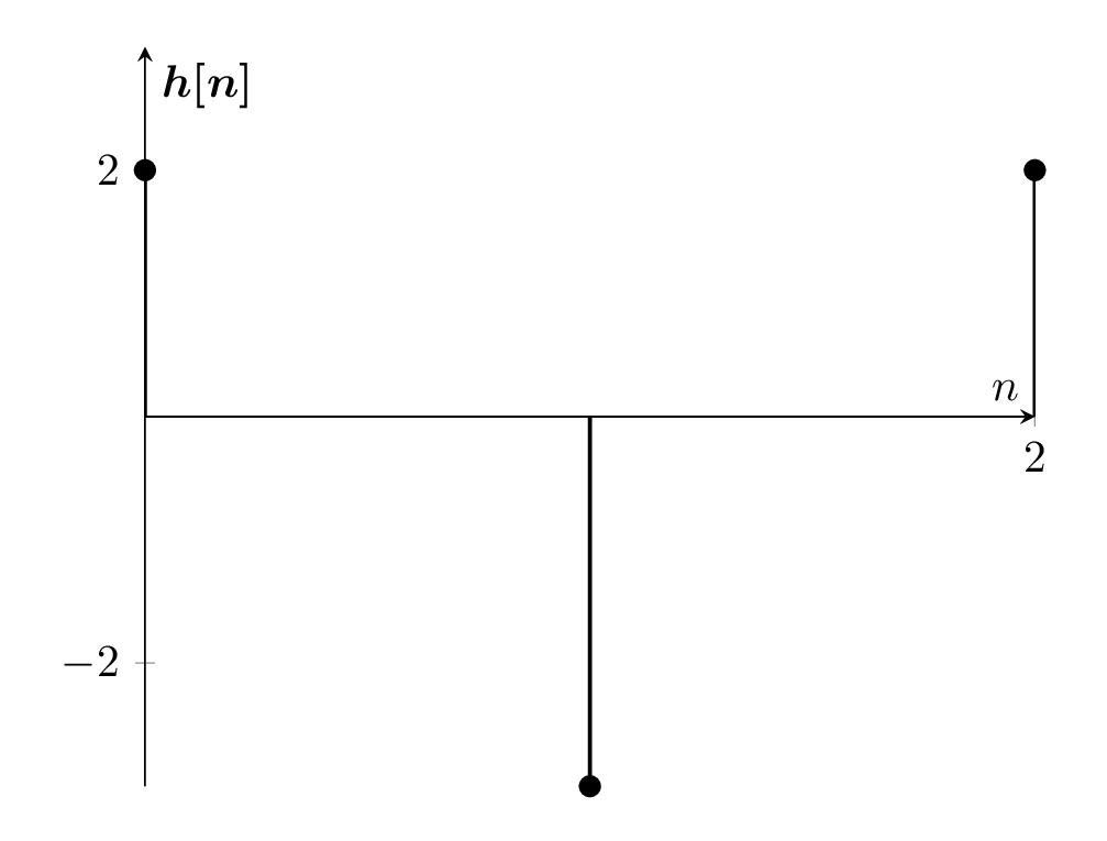
The code is a LaTeX document that includes a tikzpicture environment to create a plot of a discrete-time signal. The signal values are defined in the file data.dat using two columns: one for the index n and another for the signal value hn. The tikzpicture environment includes an axis environment that defines the x and y axes, their labels, and some other properties such as the tick marks and the y-axis limits. Finally, the signal is plotted using the addplot command with the ycomb option to create a stem plot, and the data is loaded from the file data.dat using the table command with the x and y columns specified.
Keywords
tikz, pgfplots, filecontents, amsmath, axis, ycomb, table, xtick, xlabel, ylabel, ymin, ymax, n, hn.
Source Code
\documentclass[border={10pt}]{standalone}
\usepackage{tikz,pgfplots,filecontents,amsmath}
\pgfplotsset{compat=1.5}

\begin{filecontents}{data.dat}
 n   hn
 0   2
 1   -3
 2   2.0
% 3   0.0
 %4   0.0
% 5   0.0
\end{filecontents}


\begin{document}

\begin{tikzpicture}
\begin{axis}
[%%%%%%%%%%%%%%%%%%%%%%%%%%%%%%%%%%%
    axis x line=middle,
    axis y line=middle,
    every axis x label={at={(current axis.right of origin)},anchor=north west},
    every axis y label={at={(current axis.above origin)},anchor= north west},
    every axis plot post/.style={mark options={fill=black}},
    xlabel={$n$},
    ylabel={$\boldsymbol{h[n]}$},
    xtick={-1,0,2,4},
    ymin=-3,
    ymax=3,
]%%%%%%%%%%%%%%%%%%%%%%%%%%%%%%%%%%%
\addplot+[ycomb,black,thick] table [x={n}, y={hn}] {data.dat};
\end{axis}
\end{tikzpicture}

\end{document}