Description
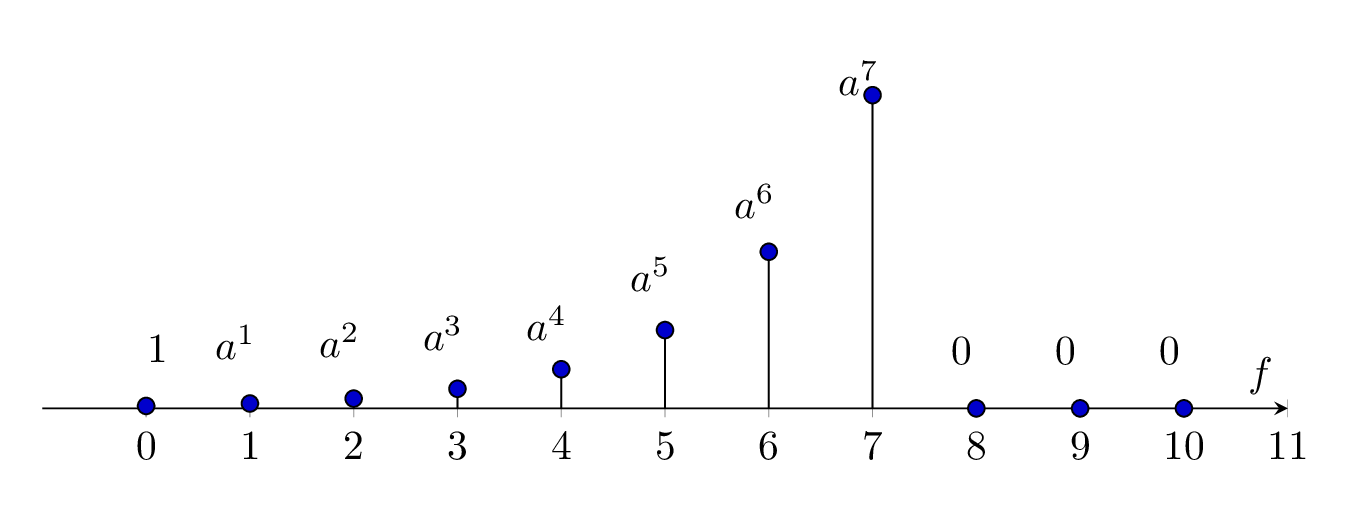
This code is a LaTeX document that generates a TikZ picture of a signal spectrum plot. It uses the pgfplots package to draw the graph and the amsmath package for math symbols. The code sets various properties of the axis, such as its height, width, x and y axis lines, and labels for the x axis. It then plots a signal spectrum using the \addplot command with ycomb style, which draws a comb-like line with y values at discrete x values. The x and y values for the plot are given in the form of coordinates. The code also includes nodes with labels at specific x and y coordinates using the \node command to annotate the graph. Finally, the document is closed with \end{document}.
Keywords
tikz, pgfplots, filecontents, amsmath, standalone, axis, xcomb, plot coordinates, node
Source Code
\documentclass[border={10pt}]{standalone}
\usepackage{tikz,pgfplots,filecontents,amsmath}
\pgfplotsset{compat=1.5}

\begin{document}

\begin{tikzpicture}
\begin{axis}
[%%%%%%%%%%%%%%%%%%%%%%%%%%%%%%%%%%%
height=5cm,
width=\textwidth,
    axis x line=middle,
    axis y line= none,
%    ylabel={Signal Spectrum of $x(t)$},
     every axis x label={at={(current axis.left of origin)},anchor=south west},
%    every axis y label={at={(current axis.above origin)},anchor= north west},
    %every axis plot post/.style={mark options={fill=black}},
    % every axis plot/.append style={ultra thick},
   xlabel={$f$},
%    ylabel={$\boldsymbol{x[n]}$},
    xtick={0,1,...,11},
    ymax=150,
    xmax=11,
    xmin=-1,
]%%%%%%%%%%%%%%%%%%%%%%%%%%%%%%%%%%%
%\addplot+[ycomb,black,thick] table [x={n}, y={xn}] {data.dat};
\addplot+[ycomb,black] plot coordinates
{(0,1) (1,2) (2,4) (3,8) (4,16) (5,32) (6,64) (7,128) (8,0) (9,0) (10,0)};
\node[label={{$1$}}] at (axis cs:0.25,1) {};
\node[label={{$a^{1}$}}] at (axis cs:1,2) {};
\node[label={{$a^{2}$}}] at (axis cs:2,3) {};
\node[label={{$a^{3}$}}] at (axis cs:3,6) {};
\node[label={{$a^{4}$}}] at (axis cs:4,10) {};
\node[label={{$a^{5}$}}] at (axis cs:5,30) {};
\node[label={{$a^{6}$}}] at (axis cs:6,60) {};
\node[label={{$a^{7}$}}] at (axis cs:7,110) {};
\node[label={{$0$}}] at (axis cs:8,0) {};
\node[label={{$0$}}] at (axis cs:9,0) {};
\node[label={{$0$}}] at (axis cs:10,0) {};
\end{axis}
\end{tikzpicture}

\end{document}