Description

% latex diagram produces diagram for the following question
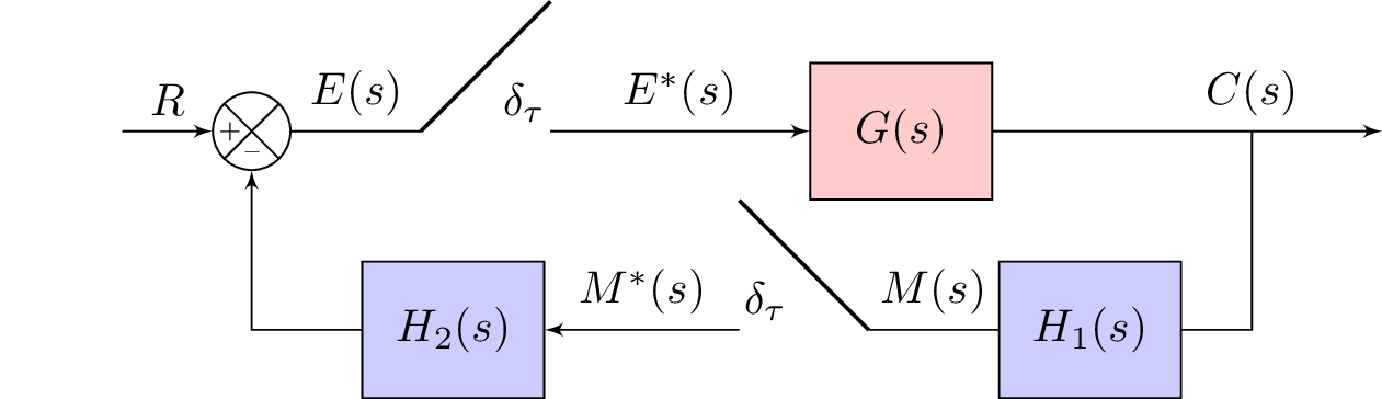
% Obtain the closed-loop pulse transfer function of the system shown in the figure below.
% Final Answer:
% 
% \begin{align*}
% & C^\ast(s) = \frac{G_2^\ast(s)G_1^\ast(s)R^\ast(s)}{1 +G_2^\ast(s)+G_1^\ast(s)
%  \left[G_2H(s)\right]^\ast} \quad  C(z) =  \frac{R(z)G_2(z) G_1(z)}{1 +G_2(z)+G_1(z)
%  \left[G_2H(z)\right]} %\\
% \end{align*}
 
\documentclass{standalone}
\usepackage{tikz}
\usetikzlibrary{positioning}
\usetikzlibrary{shapes,arrows,calc} 
\usetikzlibrary{decorations.text}
\tikzset{add/.style n args={4}{
		minimum width=6mm,
		path picture={
			\draw[black] 
			(path picture bounding box.south east) -- (path picture bounding box.north west)
			(path picture bounding box.south west) -- (path picture bounding box.north east);
			\node at ($(path picture bounding box.south)+(0,0.13)$)     {\tiny #1};
			\node at ($(path picture bounding box.west)+(0.13,0)$)      {\tiny #2};
			\node at ($(path picture bounding box.north)+(0,-0.13)$)        {\tiny #3};
			\node at ($(path picture bounding box.east)+(-0.13,0)$)     {\tiny #4};
		}
	}
}
\begin{document}
	
%\begin{figure}
%\centering
	\tikzstyle{block} = [draw, fill=blue!20, rectangle, minimum height=3em, minimum width=4em]
	\tikzstyle{controller} = [draw, fill=red!20, rectangle, minimum height=3em, minimum width=4em]
	\tikzstyle{sum} = [draw, fill=blue!20, circle, node distance=1cm]
	\tikzstyle{input} = [coordinate]
	\tikzstyle{output} = [coordinate]
	\tikzstyle{sampleSP} = [coordinate]
	\tikzstyle{sampleEP} = [coordinate]
	\tikzstyle{otherPoint} = [coordinate]
	\begin{tikzpicture}[auto, >=latex']
	% Nodes
	\node [input] (input) {};
	%\node [sum, right = 1cm of input] (sum) {};
	\node[draw,circle,add={--}{+}{}{},right of= input](sum){}; 
	\node [sampleSP, right = 1cm of sum] (sumSP) {};
	\node [sampleEP, right = 1cm of sumSP] (sumEP) {};
	\node [sampleEP, above = 1cm of sumEP] (sumEPTOP) {};
	\node [controller, right = 2cm of sumEP] (system) {$G(s)$};
	\node [otherPoint,right = 1cm of system] (branchPoint) {};
	\node [otherPoint,below = 1 cm of system] (belowsystem) {}; %{$\frac{1}{Ts+1}$};
	%\node [block, right = 1cm of system] (system2) {$\frac{1}{Ts+1}$};
	\node [output, right = 2cm of branchPoint] (output) {};
	%\node [input, below = 0.5cm of system] (m) {};
	\node [block, right = 0.75 of belowsystem] (systemH) {$H_1(s)$};
	
	% Second Sampler Point
	\node [sampleSP, left = 1cm of systemH] (sysHSP2) {};
	\node [sampleEP, left = 1cm of sysHSP2] (sysHEP2) {};
	\node [sampleEP, above = 1cm of sysHEP2] (sumEPTOP2) {};
	
	% Second block 
	\node [block, left = 1.5cm of sysHEP2] (systemH2) {$H_2(s)$};
	% Arrows
	\draw [draw,->] (input) -- node {$R$} (sum);
	% Arrows for first sampler
	\draw [-] (sum) -- node {$E(s)$} (sumSP);
	\draw [-,thick] (sumEPTOP) -- node {$\delta_\tau$} (sumSP);
	\draw [->] (sumEP) -- node {$E^\ast(s)$} (system);
	%Arrows for second sampler (bottom)
	\draw [-]  (sysHSP2)-- node {$M(s)$} (systemH);  
	\draw [-,thick] (sysHSP2) -- node {$\delta_\tau$} (sumEPTOP2);
	%\draw [->] (sumEP) -- node {$M^\ast(s)$} (systemH);
	% \draw [->] (system) --  (system2);
	\draw [-] (system) --  (branchPoint);
	\draw [->] (branchPoint) -- node (y) {$C(s)$}(output);
	\draw [-] (y) |- (systemH) {};
	%\draw [-] (y) |- (m) {} ;
	\draw [<-] (systemH2) -- node {$M^\ast(s)$} (sysHEP2);
	\draw [->] (systemH2) -| (sum); %{$-$}  node [near end] {} (sum);
	%\draw [->] (m) -| node[pos=0.99] {} node [near end] {} (sum); %{$-$}  node [near end] {} (sum);
	\end{tikzpicture}
%\end{figure}
\end{document}