Description

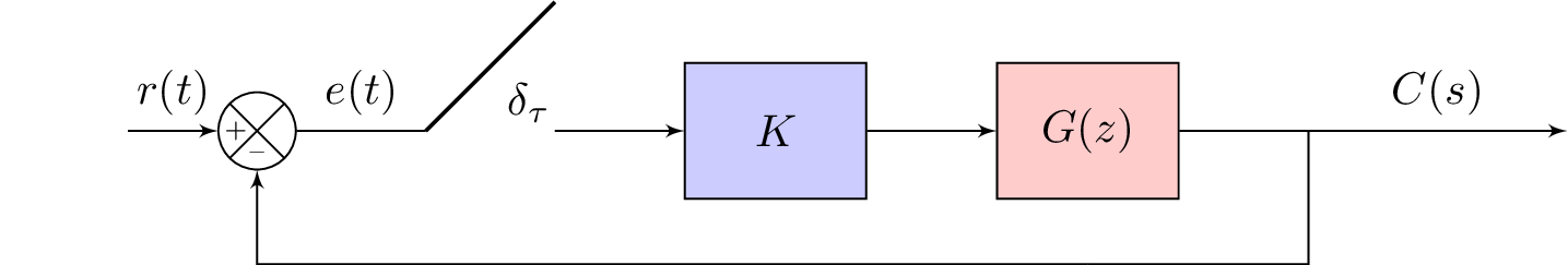
The given diagram seems to be a digital control system which consists of a feedback loop. The signal $r(t)$ is the reference signal and $y(t)$ is the output signal. The system involves a digital controller $G(z)$ , and a plant with a transfer function $K$ .

The first block in the system is the summing block which takes the reference signal $r(t)$ and the feedback signal $y(t)$ , computes their difference $e(t)$ , and provides this error signal as an input to the controller.

The controller $G(z)$ is responsible for generating the control signal to be applied to the plant. The plant has a transfer function of $K$ . The output of the plant is fed back through the summing block to generate the feedback signal $y(t)$ , which is subtracted from the reference signal to compute the error signal $e(t)$ .

The system also has two sampling points, indicated by the dotted lines with labels $\delta\_\tau$ . These sampling points indicate the instants at which the reference signal and the feedback signal are sampled and held constant for one sampling period $\tau$ .

Keywords

tikzpicture, node, draw, fill, rectangle, circle, path, coordinate, label, above, left, right, below.

Source Code

ControlSystems/CSII

 
\documentclass{standalone}
\usepackage{tikz}
\usetikzlibrary{positioning}
\usetikzlibrary{shapes,arrows,calc} 
\usetikzlibrary{decorations.text}
\tikzset{add/.style n args={4}{
		minimum width=6mm,
		path picture={
			\draw[black] 
			(path picture bounding box.south east) -- (path picture bounding box.north west)
			(path picture bounding box.south west) -- (path picture bounding box.north east);
			\node at ($(path picture bounding box.south)+(0,0.13)$)     {\tiny #1};
			\node at ($(path picture bounding box.west)+(0.13,0)$)      {\tiny #2};
			\node at ($(path picture bounding box.north)+(0,-0.13)$)        {\tiny #3};
			\node at ($(path picture bounding box.east)+(-0.13,0)$)     {\tiny #4};
		}
	}
}
\begin{document}
	
%\begin{figure}
%\centering
	\tikzstyle{block} = [draw, fill=blue!20, rectangle, minimum height=3em, minimum width=4em]
	\tikzstyle{controller} = [draw, fill=red!20, rectangle, minimum height=3em, minimum width=4em]
	\tikzstyle{sum} = [draw, fill=blue!20, circle, node distance=1cm]
	\tikzstyle{input} = [coordinate]
	\tikzstyle{output} = [coordinate]
	\tikzstyle{sampleSP} = [coordinate]
	\tikzstyle{sampleEP} = [coordinate]
	\tikzstyle{otherPoint} = [coordinate]
	\begin{tikzpicture}[auto, >=latex']
	% Nodes
	\node [input] (input) {};
	%\node [sum, right = 1cm of input] (sum) {};
	\node[draw,circle,add={--}{+}{}{},right of= input](sum){}; 
	\node [sampleSP, right = 1cm of sum] (sumSP) {};
	\node [sampleEP, right = 1cm of sumSP] (sumEP) {};
	\node [sampleEP, above = 1cm of sumEP] (sumEPTOP) {};
	\node [block, right = 1 cm of sumEP] (systemK) {$K$};
	%\node [block, right = 1 cm of systemK] (system2) {$\frac{1-e^{-s}}{s}$};
	%\node [controller, right = 1 cm of systemK] (system3) {$\frac{1}{s+1}$};
	\node [controller, right = 1 cm of systemK] (systemEND) {$G(z)$};
	\node [otherPoint,right = 1 cm of systemEND] (branchPoint) {};
	\node [otherPoint,below = 1 cm of systemEND] (belowsystem) {}; %{$\frac{1}{Ts+1}$};
	%\node [block, right = 1cm of system] (system2) {$\frac{1}{Ts+1}$};
	\node [output, right = 2cm of branchPoint] (outputY) {};
	\node [input, below = 0.5cm of systemEND] (m) {};
%	\node [block, right = 0.75 of belowsystem] (systemH) {$H_1(s)$};
	
	% Second Sampler Point
%	\node [sampleSP, left = 1cm of systemH] (sysHSP2) {};
%	\node [sampleEP, left = 1cm of sysHSP2] (sysHEP2) {};
%	\node [sampleEP, above = 1cm of sysHEP2] (sumEPTOP2) {};
	
	% Second block 
%	\node [block, left = 1.5cm of sysHEP2] (systemH2) {$H_2(s)$};
%	% Arrows
	\draw [draw,->] (input) -- node {$r(t)$} (sum);
%	% Arrows for first sampler
	\draw [-] (sum) -- node {$e(t)$} (sumSP);
	\draw [-,thick] (sumEPTOP) -- node {$\delta_\tau$} (sumSP);
	% Arrows for block diagrams
	\draw [->] (sumEP) -- node {} (systemK);
	\draw [->] (systemK) -- node {} (systemEND);
	%\draw [->] (system2) -- node {} (systemEND);
	%\draw [->] (system3) -- node {} (systemEND);
%	%Arrows for second sampler (bottom)
%	\draw [-]  (sysHSP2)-- node {$M(s)$} (systemH);  
%	\draw [-,thick] (sysHSP2) -- node {$\delta_\tau$} (sumEPTOP2);
%	%\draw [->] (sumEP) -- node {$M^\ast(s)$} (systemH);
%	% \draw [->] (system) --  (system2);
	% G(s) to branchpoint
	\draw [-] (systemEND) --  (branchPoint);
	\draw [->] (branchPoint) -- node (y) {$C(s)$}(outputY);
	%\draw [-] (outputY) |- (system) {};
	\draw [-] (branchPoint) |- (m) {} ;
%	\draw [<-] (systemH2) -- node {$M^\ast(s)$} (sysHEP2);
%	\draw [->] (systemH2) -| (sum); %{$-$}  node [near end] {} (sum);
	\draw [->] (m) -| node[pos=0.99] {} node [near end] {} (sum); %{$-$}  node [near end] {} (sum);
	\end{tikzpicture}
%\end{figure}
\end{document}

Deploy to Overleaf

Poleszeroes Sampler413