Description
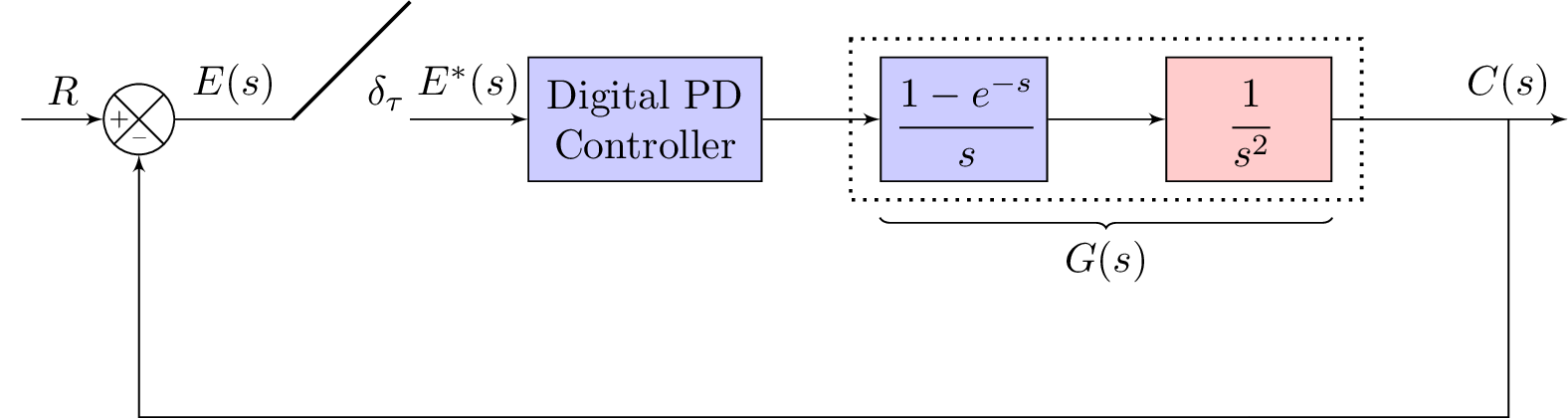
The code is a LaTeX document that generates a diagram using the TikZ package. The diagram is a block diagram that shows a closed-loop control system with a digital PD controller, a zero-order hold (ZOH), and a second-order transfer function. The diagram includes various nodes and arrows that connect the nodes, which are defined using TikZ styles. The diagram also includes labels for the nodes, which are defined using the TikZ library decorations.text.
The diagram starts with an input node, followed by a summing junction represented by a circle with a plus and a minus sign inside it. The output of the summing junction is fed into a sampler, represented by a vertical line with two horizontal lines at its top and bottom. The output of the sampler is fed into the digital PD controller, which is represented by a rectangular block. The output of the digital PD controller is then fed into a ZOH, represented by a rectangular block with a transfer function written inside it.
The output of the ZOH is fed into a second-order transfer function represented by a rectangular block with a transfer function written inside it. The output of the second-order transfer function is fed into a branch point, which then splits the signal into two paths. One path leads to the output node, while the other path leads to a feedback loop represented by a line with a small circle at its end. The feedback loop connects to the summing junction and the input node.
The diagram also includes various coordinate nodes, represented by empty circles, that help in positioning the other nodes and arrows. The diagram is enclosed in a dotted rectangle, which is defined using TikZ decorations.pathreplacing library.
Keywords
rectangle, draw, fill, node, above, right, left, below, inner sep.
Source Code
\documentclass[%
% border=1pt
border={-25pt 0pt 0pt 0pt} % left bottom right top
]{standalone}
\usepackage{tikz}
\usepackage{amsmath}
\usetikzlibrary{positioning}
\usetikzlibrary{shapes,arrows,calc}
\usetikzlibrary{decorations.text}
\usetikzlibrary{decorations.pathreplacing}
\tikzset{add/.style n args={4}{
		minimum width=6mm,
		path picture={
			\draw[black]
			(path picture bounding box.south east) -- (path picture bounding box.north west)
			(path picture bounding box.south west) -- (path picture bounding box.north east);
			\node at ($(path picture bounding box.south)+(0,0.13)$)     {\tiny #1};
			\node at ($(path picture bounding box.west)+(0.13,0)$)      {\tiny #2};
			\node at ($(path picture bounding box.north)+(0,-0.13)$)        {\tiny #3};
			\node at ($(path picture bounding box.east)+(-0.13,0)$)     {\tiny #4};
		}
	}
}
\begin{document}

%\begin{figure}
%\centering
	\tikzstyle{block} = [draw, fill=blue!20, rectangle, minimum height=3em, minimum width=4em]
	\tikzstyle{controller} = [draw, fill=red!20, rectangle, minimum height=3em, minimum width=4em]
	\tikzstyle{sum} = [draw, fill=blue!20, circle, node distance=1cm]
	\tikzstyle{input} = [coordinate]
	\tikzstyle{output} = [coordinate]
	\tikzstyle{sampleSP} = [coordinate]
	\tikzstyle{sampleEP} = [coordinate]
	\tikzstyle{otherPoint} = [coordinate]
	\tikzset{
		position label/.style={
			below = 3pt,
			text height = 1.5ex,
			text depth = 1ex
		},
		brace/.style={
			decoration={brace, mirror},
			decorate
		}
	}
	\begin{tikzpicture}[auto, >=latex']
	% Nodes
	\node [input] (input) {};
	%\node [sum, right = 1cm of input] (sum) {};
	\node[draw,circle,add={--}{+}{}{},right of= input](sum){};
	\node [sampleSP, right = 1cm of sum] (sumSP) {};
	\node [sampleEP, right = 1cm of sumSP] (sumEP) {};
	\node [sampleEP, above = 1cm of sumEP] (sumEPTOP) {};
	\node [block, right = 1cm of sumEP,text width=1.75cm,align=center] (systemK) {Digital PD Controller};
	\node [block, right = 1cm of systemK] (systemZOH) {$\cfrac{1-e^{-s}}{s}$};
	\node [controller, right = 1cm of systemZOH] (system) {$\cfrac{1}{s^2}$};
	\node [otherPoint,right = 1cm of system] (branchPoint) {};
	\node [otherPoint,below = 1 cm of system] (belowsystem) {}; %{$\frac{1}{Ts+1}$};
	%\node [block, right = 1cm of system] (system2) {$\frac{1}{Ts+1}$};
	\node [output, right = 1cm of branchPoint] (output) {};
	\node [input, below = 2cm of system] (m) {};

	% Arrows
	\draw [draw,->] (input) -- node {$R$} (sum);
	% Arrows for first sampler
	\draw [-] (sum) -- node {$E(s)$} (sumSP);
	\draw [-,thick] (sumEPTOP) -- node {$\delta_\tau$} (sumSP);
	\draw [->] (sumEP) -- node {$E^\ast(s)$} (systemK);
	\draw [->] (systemK) -- node {} (systemZOH);
	\draw [->] (systemZOH) -- node {} (system);
	%\draw [->] (sumEP) -- node {$M^\ast(s)$} (systemH);
	% \draw [->] (system) --  (system2);
	\draw [-] (system) --  (branchPoint);
	\draw [->] (branchPoint) -- node (y) {$C(s)$}(output);

	\draw [-] (y) |- (m) {} ;
	\draw [->] (m) -| (sum); %{$-$}  node [near end] {} (sum);
	%\node [below = 0.005 cm of system] (PointHeader) {\scriptsize{$G(s)$}};
	\draw[thick,dotted]     ($(systemZOH.north west)+(-0.25,0.15)$) rectangle ($(system.south east)+(0.25,-0.15)$);
	\draw [brace,decoration={raise=2ex}] (systemZOH.south west) -- node [position label,yshift=-2ex] {$G(s)$} (system.south east);
	\end{tikzpicture}
%\end{figure}
\end{document}