Description
This is a LaTeX code that produces a 3D diagram and two equations with descriptions.
The document class is standalone, which generates a tightly cropped output without margins. The packages tikz and bm are loaded. The ragged2e package with the option raggedrightboxes is also included.
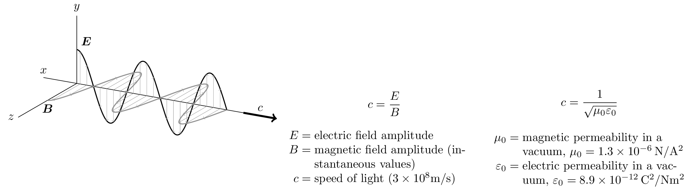
The code starts by defining the 3D environment using the tikzpicture environment with the x, y, and z axis directions. The axes are drawn using the draw command with different line styles and colors. A propagation vector is also drawn using the draw and node commands.
Two different waves are then plotted using the plot command with a domain and a number of samples. Two arrows are also drawn for each point on the wave using a foreach loop.
Two labeled nodes, and , are added using the node command.
The second part of the code contains two minipage environments. The first one contains an equation and a table with descriptions, while the second one includes another equation and a table with descriptions.
Keywords
TikZ, 3D, wave propagation, electric field, magnetic field, speed of light, formula, table.
Source Code
\documentclass{standalone}
\usepackage{tikz,bm}
\usepackage[raggedrightboxes]{ragged2e}
\begin{document}
  \begin{tikzpicture}[x={(-10:1cm)},y={(90:1cm)},z={(210:1cm)}]
    % Axes
    \draw (-1,0,0) node[above] {$x$} -- (5,0,0);
    \draw (0,0,0) -- (0,2,0) node[above] {$y$};
    \draw (0,0,0) -- (0,0,2) node[left] {$z$};
    % Propagation
    \draw[->,ultra thick] (5,0,0) -- node[above] {$c$} (6,0,0);
    % Waves
    \draw[thick] plot[domain=0:4.5,samples=200] (\x,{cos(deg(pi*\x))},0);
    \draw[gray,thick] plot[domain=0:4.5,samples=200] (\x,0,{cos(deg(pi*\x))});
    % Arrows
    \foreach \x in {0.1,0.3,...,4.4} {
      \draw[->,help lines] (\x,0,0) -- (\x,{cos(deg(pi*\x))},0);
      \draw[->,help lines] (\x,0,0) -- (\x,0,{cos(deg(pi*\x))});
    }
    % Labels
    \node[above right] at (0,1,0) {$\bm{E}$};
    \node[below] at (0,0,1) {$\bm{B}$};
  \end{tikzpicture}

  \begin{minipage}{.5\linewidth}
    \[
      c = \frac{E}{B}
    \]
    \begin{tabular}{r@{${}={}$}p{.8\linewidth}}
      $E$ & electric field amplitude \\
      $B$ & magnetic field amplitude (instantaneous values) \\
      $c$ & speed of light ($3\times10^8\mathrm{m/s}$) \\
    \end{tabular}
  \end{minipage}%
  \begin{minipage}{.5\linewidth}
    \[
      c = \frac{1}{\sqrt{\mu_0 \varepsilon_0}}
    \]
    \begin{tabular}{r@{${}={}$}p{.8\linewidth}}
      $\mu_0$ & magnetic permeability in a vacuum, $\mu_0 = 1.3\times10^{-6}\,\mathrm{N/A^2}$ \\
      $\varepsilon_0$ & electric permeability in a vacuum, $\varepsilon_0 = 8.9\times10^{-12}\,\mathrm{C^2/N m^2}$ \\
    \end{tabular}
  \end{minipage}
\end{document}