Description
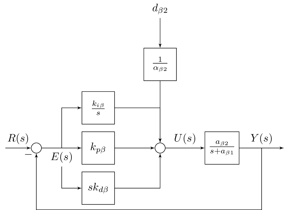
The code above is a TikZ code for drawing a PID control system block diagram. The diagram consists of several blocks and arrows representing the flow of signals in the system.
The blocks in the diagram are defined using TikZ styles, which specify their appearance and properties. These include a block style for rectangular blocks, a sum style for circular summing junctions, an input style for input signals, an output style for output signals, and pinstyle for adding labels to the arrows.
The main components of the diagram include an input node representing the input signal, a summing junction node for calculating the error signal, a controller block for implementing the PID control algorithm, a rate block for the derivative action, an extra block that is used to add a feedforward term, a system block representing the process or plant being controlled, and an output node representing the output signal.
The arrows connecting the blocks represent the flow of signals between the various components of the system. For example, there is an arrow connecting the input node to the summing junction node to represent the input signal, and there is an arrow connecting the output node to the system block to represent the output signal.
Overall, the code generates a professional-looking block diagram that can be used for educational or presentation purposes in the field of control engineering.
Keywords
tikz, shapes, arrows, positioning, calc, block, tmp, sum, input, output, pinstyle.
Source Code
\documentclass{standalone}
\usepackage{tikz}
\usetikzlibrary{shapes,arrows,positioning,calc}

\begin{document}

	\tikzset{
		block/.style = {draw, fill=white, rectangle, minimum height=3em, minimum width=3em},
		tmp/.style  = {coordinate},
		sum/.style= {draw, fill=white, circle, node distance=1cm},
		input/.style = {coordinate},
		output/.style= {coordinate},
		pinstyle/.style = {pin edge={to-,thin,black}
		}
	}


	%\begin{figure}[!htb]
	%\centering
	\begin{tikzpicture}[auto, node distance=2cm,>=latex']
	\node [input, name=rinput] (rinput) {};
	\node [sum, right of=rinput] (sum1) {};
	\node [block, right of=sum1] (controller) {$k_{p\beta}$};
	\node [block, above of=controller,node distance=1.3cm] (up){$\frac{k_{i\beta}}{s}$};
	\node [block, below of=controller,node distance=1.3cm] (rate) {$sk_{d\beta}$};
	\node [sum, right of=controller,node distance=2cm] (sum2) {};
	\node [block, above = 2cm of sum2](extra){$\frac{1}{\alpha_{\beta2}}$};  %
	\node [block, right of=sum2,node distance=2cm] (system)
	{$\frac{a_{\beta 2}}{s+a_{\beta 1}}$};
	\node [output, right of=system, node distance=2cm] (output) {};
	\node [tmp, below of=controller] (tmp1){$H(s)$};
	\draw [->] (rinput) -- node{$R(s)$} (sum1);
	\draw [->] (sum1) --node[name=z,anchor=north]{$E(s)$} (controller);
	\draw [->] (controller) -- (sum2);
	\draw [->] (sum2) -- node{$U(s)$} (system);
	\draw [->] (system) -- node [name=y] {$Y(s)$}(output);
	\draw [->] (z) |- (rate);
	\draw [->] (rate) -| (sum2);
	\draw [->] (z) |- (up);
	\draw [->] (up) -| (sum2);
	\draw [->] (y) |- (tmp1)-| node[pos=0.99] {$-$} (sum1);
	\draw [->] (extra)--(sum2);
	\draw [->] ($(0,1.5cm)+(extra)$)node[above]{$d_{\beta 2}$} -- (extra);
	\end{tikzpicture}
	%\caption{A PID Control System} \label{fig6_10}
	%\end{figure}

\end{document}