Description
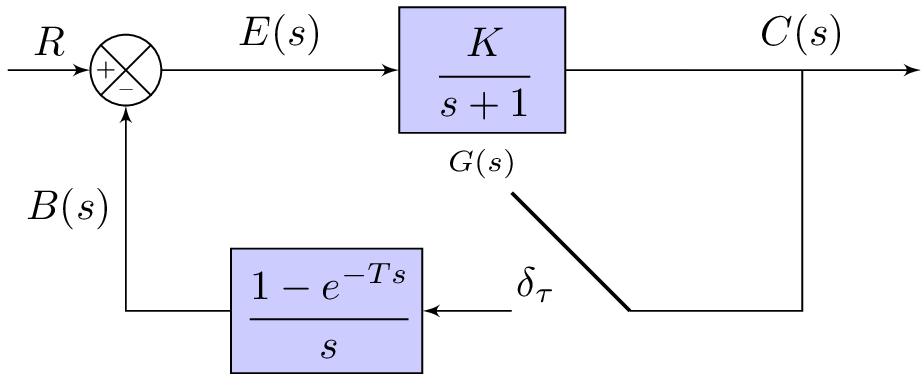
The code is a LaTeX document that generates a block diagram using the TikZ package. The block diagram depicts a closed-loop control system consisting of a controller, a plant, and feedback. The diagram includes several components such as summing junctions, blocks, and signals.
The code defines various TikZ styles for different types of nodes such as "block", "controller", "sum", "input", "output", "sampleSP", "sampleEP", and "otherPoint". These styles define the appearance of the corresponding nodes in the block diagram. For example, the "block" style sets the node shape to a rectangle with a blue fill, while the "sum" style sets the node shape to a circle with a blue fill.
The code then defines the nodes of the block diagram and connects them using arrows. The nodes include an input node, a summing junction node, a plant block node, an output node, and other miscellaneous nodes. The arrows between the nodes represent the flow of signals through the system.
Finally, the code specifies the layout of the nodes using the TikZ "positioning" library. This allows the user to specify the relative positioning of the nodes with respect to each other.
Keywords
tikzpicture, node, rectangle, draw, align, below, left, right, text width, fill, black, minimum height, minimum width, anchor, east, west.
Source Code
\documentclass[%
% border=1pt
border={-25pt 0pt 0pt 0pt} % left bottom right top
]{standalone}
\usepackage{amsmath}
\usepackage{tikz}
\usetikzlibrary{positioning}
\usetikzlibrary{shapes,arrows,calc}
\usetikzlibrary{decorations.text}
\tikzset{add/.style n args={4}{
		minimum width=6mm,
		path picture={
			\draw[black]
			(path picture bounding box.south east) -- (path picture bounding box.north west)
			(path picture bounding box.south west) -- (path picture bounding box.north east);
			\node at ($(path picture bounding box.south)+(0,0.13)$)     {\tiny #1};
			\node at ($(path picture bounding box.west)+(0.13,0)$)      {\tiny #2};
			\node at ($(path picture bounding box.north)+(0,-0.13)$)        {\tiny #3};
			\node at ($(path picture bounding box.east)+(-0.13,0)$)     {\tiny #4};
		}
	}
}
\begin{document}

%\begin{figure}
%\centering
	\tikzstyle{block} = [draw, fill=blue!20, rectangle, minimum height=3em, minimum width=4em]
	\tikzstyle{controller} = [draw, fill=red!20, rectangle, minimum height=3em, minimum width=4em]
	\tikzstyle{sum} = [draw, fill=blue!20, circle, node distance=1cm]
	\tikzstyle{input} = [coordinate]
	\tikzstyle{output} = [coordinate]
	\tikzstyle{sampleSP} = [coordinate]
	\tikzstyle{sampleEP} = [coordinate]
	\tikzstyle{otherPoint} = [coordinate]
	\begin{tikzpicture}[auto, >=latex']
	% Nodes
	\node [input] (input) {};
	%\node [sum, right = 1cm of input] (sum) {};
	\node[draw,circle,add={--}{+}{}{},right of= input](sum){};
	%\node [sampleSP, right = 1cm of sum] (sumSP) {};
	%\node [sampleEP, right = 1cm of sumSP] (sumEP) {};
	%\node [sampleEP, above = 1cm of sumEP] (sumEPTOP) {};
	\node [block, right = 2cm of sum] (system) {$\cfrac{K}{s+1}$}; % node[label=below:$b_1$,draw]{};
	\node [below = 0.005 cm of system] (PointHeader) {\scriptsize{$G(s)$}};
	\node [otherPoint,right = 1cm of system] (branchPoint) {};
	\node [otherPoint,below = 1 cm of system] (belowsystem) {}; %{$\frac{1}{Ts+1}$};
	%\node [block, right = 1cm of system] (system2) {$\frac{1}{Ts+1}$};
	\node [output, right = 2cm of branchPoint] (output) {};
	%\node [input, below = 0.5cm of system] (m) {};
	\node [otherPoint, right = 1.25 of belowsystem] (systemRightDownP) {$H_1(s)$};

	% Second Sampler Point
	\node [sampleSP, below = 0.5cm of systemRightDownP] (sysHSP2) {};
	\node [sampleEP, left = 1cm of sysHSP2] (sysHEP2) {};
	\node [sampleEP, above = 1cm of sysHEP2] (sumEPTOP2) {};

	% Second block
	\node [block, left = 0.75cm of sysHEP2] (systemH2) {$\cfrac{1-e^{-Ts}}{s}$};
	% Arrows
	\draw [draw,->] (input) -- node {$R$} (sum);
	% Arrows for first sampler
%	\draw [-] (sum) -- node {$E(s)$} (sumSP);
%	\draw [-,thick] (sumEPTOP) -- node {$\delta_\tau$} (sumSP);
	\draw [->] (sum) -- node {$E(s)$} (system);
	%Arrows for second sampler (bottom)
%	\draw [-]  (sysHSP2)-- node {$M(s)$} (systemH);
	\draw [-,thick] (sysHSP2) -- node {$\delta_\tau$} (sumEPTOP2);
	%\draw [->] (sumEP) -- node {$M^\ast(s)$} (systemH);
	% \draw [->] (system) --  (system2);
	\draw [-] (system) --  (branchPoint);
	\draw [->] (branchPoint) -- node (y) {$C(s)$}(output);
	\draw [-] (y) |- (sysHSP2) {};
	%\draw [-] (y) |- (m) {} ;
	%\draw [<-] (systemH2) -- node {$M^\ast(s)$} (sysHEP2);
	\draw [->] (sysHEP2) -- (systemH2);
	\draw [->] (systemH2) -| node [near end] {$B(s)$} (sum) ; %{$-$}  node [near end] {} (sum);
	%\node [otherPoint, below = 1.25cm of sum] (Text) {$B(s)$};
	%\draw [->] (m) -| node[pos=0.99] {} node [near end] {} (sum); %{$-$}  node [near end] {} (sum);
	\end{tikzpicture}
%\end{figure}
\end{document}