Description
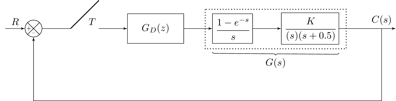
The code is a LaTeX document that uses the standalone class to produce a standalone figure. The figure is a block diagram of a control system and is created using the tikz package for drawing graphics in LaTeX.
The code starts by defining several styles for the different elements in the block diagram, such as block for rectangular blocks, sum for circles with a plus sign inside, input and output for coordinates representing the input and output of the system, and sampleSP and sampleEP for coordinates representing the start and end of a sample period.
The add style is also defined, which is a custom style used to add plus and minus signs to circles. The brace style is defined to add a brace decoration to a path.
The actual block diagram is then drawn using a tikzpicture environment. Nodes are created for each element in the diagram, such as the input, summing junction, system blocks, and output. Arrows are then drawn between the nodes to represent the flow of signals in the system.
Finally, some formatting options are added, such as labels for the arrows and some whitespace around the diagram. The resulting output is a standalone image of the control system block diagram.
Keywords
tikz, nodes, edges, styles, arrow tips, positioning, shapes, colors.
Source Code
\documentclass[%
% border=1pt
border={-25pt 0pt 0pt 0pt} % left bottom right top
]{standalone}
\usepackage{tikz}
\usepackage{amsmath}
\usetikzlibrary{positioning}
\usetikzlibrary{shapes,arrows,calc}
\usetikzlibrary{decorations.text}
\usetikzlibrary{decorations.pathreplacing}
\tikzset{add/.style n args={4}{
		minimum width=6mm,
		path picture={
			\draw[black]
			(path picture bounding box.south east) -- (path picture bounding box.north west)
			(path picture bounding box.south west) -- (path picture bounding box.north east);
			\node at ($(path picture bounding box.south)+(0,0.13)$)     {\tiny #1};
			\node at ($(path picture bounding box.west)+(0.13,0)$)      {\tiny #2};
			\node at ($(path picture bounding box.north)+(0,-0.13)$)        {\tiny #3};
			\node at ($(path picture bounding box.east)+(-0.13,0)$)     {\tiny #4};
		}
	}
}
\begin{document}

%\begin{figure}
%\centering
	%\tikzstyle{block} = [draw, fill=blue!20, rectangle, minimum height=3em, minimum width=4em]
	\tikzstyle{block} = [draw, rectangle, minimum height=3em, minimum width=4em]
	\tikzstyle{controller} = [draw, fill=red!20, rectangle, minimum height=3em, minimum width=4em]
	\tikzstyle{sum} = [draw, fill=blue!20, circle, node distance=1cm]
	\tikzstyle{input} = [coordinate]
	\tikzstyle{output} = [coordinate]
	\tikzstyle{sampleSP} = [coordinate]
	\tikzstyle{sampleEP} = [coordinate]
	\tikzstyle{otherPoint} = [coordinate]
	\tikzset{
		position label/.style={
			below = 3pt,
			text height = 1.5ex,
			text depth = 1ex
		},
		brace/.style={
			decoration={brace, mirror},
			decorate
		}
	}
	\begin{tikzpicture}[auto, >=latex']
	% Nodes
	\node [input] (input) {};
	%\node [sum, right = 1cm of input] (sum) {};
	\node[draw,circle,add={--}{+}{}{},right of= input](sum){};
	\node [sampleSP, right = 1cm of sum] (sumSP) {};
	\node [sampleEP, right = 1cm of sumSP] (sumEP) {};
	\node [sampleEP, above = 1cm of sumEP] (sumEPTOP) {};
	\node [block, right = 1cm of sumEP,text width=1.75cm,align=center] (systemK) {$G_D(z)$};
	\node [block, right = 1cm of systemK] (systemZOH) {$\cfrac{1-e^{-s}}{s}$};
	\node [block, right = 1cm of systemZOH] (system) {$\cfrac{K}{(s)(s+0.5)}$};
	\node [otherPoint,right = 1cm of system] (branchPoint) {};
	\node [otherPoint,below = 1 cm of system] (belowsystem) {}; %{$\frac{1}{Ts+1}$};
	%\node [block, right = 1cm of system] (system2) {$\frac{1}{Ts+1}$};
	\node [output, right = 1cm of branchPoint] (output) {};
	\node [input, below = 2cm of system] (m) {};

	% Arrows
	\draw [draw,->] (input) -- node {$R$} (sum);
	% Arrows for first sampler
	%\draw [-] (sum) -- node {$E(s)$} (sumSP);
	\draw [-] (sum) -- node {} (sumSP);
	\draw [-,thick] (sumEPTOP) -- node {$T$} (sumSP);
	%\draw [->] (sumEP) -- node {$E^\ast(s)$} (systemK);
	\draw [->] (sumEP) -- node {} (systemK);

	\draw [->] (systemK) -- node {} (systemZOH);
	\draw [->] (systemZOH) -- node {} (system);
	%\draw [->] (sumEP) -- node {$M^\ast(s)$} (systemH);
	% \draw [->] (system) --  (system2);
	\draw [-] (system) --  (branchPoint);
	\draw [->] (branchPoint) -- node (y) {$C(s)$}(output);

	\draw [-] (y) |- (m) {} ;
	\draw [->] (m) -| (sum); %{$-$}  node [near end] {} (sum);
	%\node [below = 0.005 cm of system] (PointHeader) {\scriptsize{$G(s)$}};
	\draw[thick,dotted]     ($(systemZOH.north west)+(-0.25,0.15)$) rectangle ($(system.south east)+(0.25,-0.15)$);
	\draw [brace,decoration={raise=2ex}] (systemZOH.south west) -- node [position label,yshift=-2ex] {$G(s)$} (system.south east);
	\end{tikzpicture}
%\end{figure}
\end{document}