Description
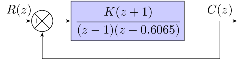
The code produces a diagram of a digital control system using the TikZ package in LaTeX. The system consists of an input node, a summing node represented by a circle with a plus and minus sign, a digital filter represented by a rectangular block with the transfer function written inside, a branch point, and an output node. The diagram also includes a node labeled "m" to represent a measurement point. The arrows connecting the nodes represent the flow of signals through the system. The code also includes annotations and calculations to determine the root loci and stability of the system for different values of gain K.
Keywords
pgfplots, addplot, domain, samples, smooth, blue, dashed, red, xlabel, ylabel, legend, legend entries.
Source Code
% Latex diagram produces diagram for the following question
% Consider the digital control system shown below. Plot the root loci as the gain K is varied from $0$ to $\infty$. Determine the critical value of gain K for stability. The sampling period is 0.1 sec, or $T=0.1$ What value of gain K will yield a damping ration $\zeta$ of the closed-loop poles equal to 0.5? With gain K set to yield $\zeta=0.5$, determine the damped natural frequency $\omega_d$ and the number of samples per cycle of damped sinusoidal oscillation.

% Numerical Answer in latex
% When $K=0.0646, \zeta=0.5$ with the pole at $z=0.771+j0.277=|0.8192|e^{j19.7620^\circ}$.
% \begin{align*}
% z=  & |e^{-T(\zeta \omega_n)} |e^{T \omega_d} = |0.8192|e^{j19.7620^\circ} \\
% & \omega_n = \frac{\ln(0.8192)}{(-0.1)(0.5)}=3.98854 = 4 \ \text{rad/s} \\
% & \omega_d = \frac{(19.7629^\circ)}{0.1} = 3.449 \quad  \omega_d = \omega_n \sqrt{1-\zeta^2}=3.988 (0.866025)=3.4537 \ \text{rad/s} \\
% & \text{Number of Samples per Cycle } = \frac{360^\circ}{T\omega_d}=\frac{360^\circ}{19.7629^\circ}=18.22
% \end{align*}

\documentclass[%
% border=1pt
border={-25pt 0pt 0pt 0pt} % left bottom right top
]{standalone}
\usepackage{amsmath}
\usepackage{tikz}
\usetikzlibrary{positioning}
\usetikzlibrary{shapes,arrows,calc}
\usetikzlibrary{decorations.text}
\tikzset{add/.style n args={4}{
		minimum width=6mm,
		path picture={
			\draw[black]
			(path picture bounding box.south east) -- (path picture bounding box.north west)
			(path picture bounding box.south west) -- (path picture bounding box.north east);
			\node at ($(path picture bounding box.south)+(0,0.13)$)     {\tiny #1};
			\node at ($(path picture bounding box.west)+(0.13,0)$)      {\tiny #2};
			\node at ($(path picture bounding box.north)+(0,-0.13)$)        {\tiny #3};
			\node at ($(path picture bounding box.east)+(-0.13,0)$)     {\tiny #4};
		}
	}
}
\begin{document}

	%\begin{figure}
	%\centering
	\tikzstyle{block} = [draw, fill=blue!20, rectangle, minimum height=3em, minimum width=4em]
	\tikzstyle{controller} = [draw, fill=red!20, rectangle, minimum height=3em, minimum width=4em]
	\tikzstyle{sum} = [draw, fill=blue!20, circle, node distance=1cm]
	\tikzstyle{input} = [coordinate]
	\tikzstyle{output} = [coordinate]
	\tikzstyle{sampleSP} = [coordinate]
	\tikzstyle{sampleEP} = [coordinate]
	\tikzstyle{otherPoint} = [coordinate]
	\begin{tikzpicture}[auto, >=latex']
	% Nodes
	\node [input] (input) {};
	%\node [sum, right = 1cm of input] (sum) {};
	\node[draw,circle,add={--}{+}{}{},right of= input](sum){};
	%\node [sampleSP, right = 1cm of sum] (sumSP) {};
	%\node [sampleEP, right = 1cm of sumSP] (sumEP) {};
	%\node [sampleEP, above = 1cm of sumEP] (sumEPTOP) {};
	\node [block, right = 0.5cm of sum] (system) {$\cfrac{K(z+1)}{(z-1)(z-0.6065)}$}; % node[label=below:$b_1$,draw]{};
	%\node [below = 0.005 cm of system] (PointHeader) {\scriptsize{$G(s)$}};
	\node [otherPoint,right = 0.5cm of system] (branchPoint) {};
	\node [otherPoint,below = 0.5 cm of system] (belowsystem) {}; %{$\frac{1}{Ts+1}$};
	%\node [block, right = 1cm of system] (system2) {$\frac{1}{Ts+1}$};
	\node [output, right = 1cm of branchPoint] (output) {};
	\node [input, below = 0.5cm of system] (m) {};
	%\node [otherPoint, right = 1.25 of belowsystem] (systemRightDownP) {$H_1(s)$};

	% Second Sampler Point
	%\node [sampleSP, below = 0.5cm of systemRightDownP] (sysHSP2) {};
	%\node [sampleEP, left = 1cm of sysHSP2] (sysHEP2) {};
	%\node [sampleEP, above = 1cm of sysHEP2] (sumEPTOP2) {};

	% Second block
	%\node [block, left = 0.75cm of sysHEP2] (systemH2) {$\cfrac{1-e^{-Ts}}{s}$};
	% Arrows
	\draw [draw,->] (input) -- node {$R(z)$} (sum);
	% Arrows for first sampler
	%	\draw [-] (sum) -- node {$E(s)$} (sumSP);
	%	\draw [-,thick] (sumEPTOP) -- node {$\delta_\tau$} (sumSP);

	%\draw [->] (sum) -- node {$E(s)$} (system);
	\draw [->] (sum) -- node {} (system);
	%Arrows for second sampler (bottom)
	%	\draw [-]  (sysHSP2)-- node {$M(s)$} (systemH);
	%\draw [-,thick] (sysHSP2) -- node {$\delta_\tau$} (sumEPTOP2);
	%\draw [->] (sumEP) -- node {$M^\ast(s)$} (systemH);
	% \draw [->] (system) --  (system2);
	\draw [-] (system) --  (branchPoint);
	\draw [->] (branchPoint) -- node (y) {$C(z)$}(output);
	%\draw [-] (y) |- (sysHSP2) {};
	\draw [-] (y) |- (m) {} ;
	%\draw [<-] (systemH2) -- node {$M^\ast(s)$} (sysHEP2);
	%\draw [->] (sysHEP2) -- (systemH2);
	%\draw [->] (systemH2) -| node [near end] {$B(s)$} (sum) ; %{$-$}  node [near end] {} (sum);
	%\node [otherPoint, below = 1.25cm of sum] (Text) {$B(s)$};
	\draw [->] (m) -| node[pos=0.99] {} node [near end] {} (sum); %{$-$}  node [near end] {} (sum);
	\end{tikzpicture}
	%\end{figure}
\end{document}